8.7.1. dasLLAMA-00 — The Problem Statement

dasLLAMA is daslang’s LLM library. It loads and runs large language models: GGUF model files, quantized weights, CPU and GPU backends, chat, speech. It is the engine behind dasllama-server. If you are here to use it, skip this page and start with tutorial 01 — a few lines of code, and a model talks to you.

Here we go the other way: before using dasLLAMA, we build the thing it has to become.

We build an inference engine. Inference means the model infers the next word from the previous ones. Training is how the model was made — a separate story.

The machine that infers is a transformer: the network design behind every modern LLM. It is a stack of identical layers. Each layer reads a list of numbers, improves it a little, and passes it on. The stack transforms its input, step by step, until the result points at the next word — that is the name. We build a complete transformer in one daslang file: about 500 lines, nothing beyond the standard library. We load a real model, run it, and complete a prompt — the text you give the model to start from.

No machine-learning background needed. By the end you should be able to read the code line by line and understand what every line does and why it is there.

8.7.1.1. Get the model

Download the two files used by Karpathy’s llama2.c:

• stories15M.bin — the model: 15 million learned numbers. Trained on TinyStories, simple children’s stories — that is why something this small can tell a coherent tale.

• tokenizer.bin — its tokenizer: turns text into the model’s tokens and back.

Put them anywhere convenient. You can run this with the interpreter at about six tokens per second, and watch the words flow:

daslang.exe tutorials/dasLLAMA/00_problem_statement.das -- stories15M.bin tokenizer.bin "Once upon a time"

Or run it with -jit at about 75, which may be more practical:

daslang.exe -jit tutorials/dasLLAMA/00_problem_statement.das -- stories15M.bin tokenizer.bin "Once upon a time"

Leave off the final argument to use the default prompt. Try different prompts — you may end up with different stories. With the default one, you get exactly this:

dim=288, layers=6, heads=6, parameters≈15204000

Once upon a time, there was a little girl named Lily. She loved to play
outside in the sunshine. One day, she saw a big, red ball in the sky. It
was the sun! She thought it was so pretty.
...

The rest of Lily’s story follows.

8.7.1.2. Numbers, not words

The model cannot read. Before it runs, a tokenizer cuts the prompt into tokens: short words or parts of words. The model knows exactly 32,000 of them — that list is its vocabulary. The count is a setting of this particular model, not a law: real models turn the same dials higher, and nothing below depends on the exact values. Once is one token; so is upon. The model receives only their integer IDs. Everything after that is arithmetic on vectors — fixed-length arrays of floats.

Where do the model’s 15 million numbers — its parameters — come from? Long before this program runs, someone showed the model text, nudged every number so the true next token scores a little higher, and repeated that a few billion times. That is training, and that is why every table and matrix below is called learned — each value was picked, example by example, so the prediction comes out right. We never train here. We only run the result.

The model’s parameters include a learned table with one row per vocabulary token — 32,000 rows, each 288 floats wide. A token ID picks its row by plain lookup, and from then on the model computes with those floats, not the ID. The row is the token’s embedding.

Tokens that behave alike get similar embeddings: dog lands much closer to cat than to Tuesday. Nobody programmed that — training pushed them together, because contexts that fit one usually fit the other. No single float means anything by itself; the pattern of all 288 together is what carries meaning.

Vectors are compared with the dot product: multiply matching coordinates and add everything up.

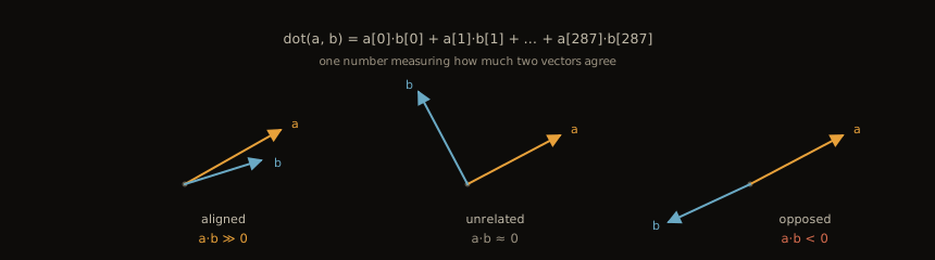
The result is one number that measures agreement, and it is the only comparison this program ever makes. The dot product depends only on the two arrows’ lengths and the angle between them — turn both by the same amount, and nothing changes.

A matrix is a stack of patterns: one learned vector per row. Multiply the matrix by an embedding and you get one dot product per row — many questions asked at once, one answer each. This is called a projection: one vector goes in, a new vector of answers comes out. Every matrix in this program works exactly this way. Nearly all the running time is this one operation.

8.7.1.3. The transformer at a glance

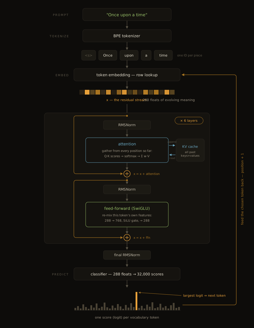
One token’s journey. The sections below walk through every box on this diagram.

x starts as the token’s embedding — the 288 floats from the table. Each of the six layers then adds two corrections to it. The first pulls in information from the tokens seen so far — this is attention, the only step where positions talk to each other. The second reworks the token’s own features, in place — this is the feed-forward block. Correction means addition: x = x + correction, twice per layer. Nothing ever replaces x; layers only add their differences on top. A running sum of differences — residuals — is why x is called the residual stream: everything the model has worked out about the current token so far.

The program’s first printed line showed three of this model’s settings; here are all of them, with the size-independent idea each one sets:

Setting	Here	The idea
dim	288	width: every stream vector is this long
layers	6	depth: how many times x gets corrected
heads	6	ways of looking back, per layer
head_size	48	dim / heads — one head’s slice of the stream
hidden	768	the feed-forward block’s wider middle, ~8/3 · dim
vocab	32000	tokens the model knows
seq_len	256	positions the model can hold

At the end we compare the result vector with every row of the embedding table — one row per vocabulary token, and the dot product again. Rows that look alike get a higher score; the score is called a logit, and the winner is the highest one. The vocabulary helps us decide — classify — what our vector is most like, and that is why this final matrix is called the classifier. The winning token then feeds back in at position + 1, and the journey repeats.

Before the model can continue our prompt, it must read it: every prompt token goes through the transformer, one after another. Each pass makes two things, about two different tokens: a stored record of the token it was given — later positions will read it — and, at the top, the logits’ guess at the token that follows. While the prompt is being read, the guess is thrown away: the next token is already in the prompt. The record is the point. This warm-up is called prefill. Then comes the loop: pick the winner, print it, feed it back, pick again — that is generation: now the guess is the point, and every generated token still leaves its record. Same transformer both times. The only difference is where the next token comes from: the prompt, or the model’s own last pick.

8.7.1.4. Five small functions

Five functions do all the math: matmul, rmsnorm, softmax, silu, rope. The first one you already know — the matrix multiplication. It takes a matrix in w, multiplies it by the vector in x, and puts the result in y:

def matmul(var y : array<float>; w : array<float>#; x : array<float>; n, d : int) {
    for (row in range(d)) {
        var sum = 0.0
        let offset = row * n
        for (col in range(n)) {
            sum += w[offset + col] * x[col]
        }
        y[row] = sum
    }
}

You can easily make it a lot faster. Much of the work in real LLM engines is exactly that: making this one loop really, really fast.

8.7.1.5. Where the weights come from

Training runs for a long time, and from time to time the trainer saves all the numbers to disk — a save point: a checkpoint. The file we downloaded is one such save. Inside is one flat array of 32-bit floats with a seven-integer header in front. The embedding table, every attention matrix, every feed-forward matrix, the classifier — all slices of that one array, at offsets the header determines. We map the file into memory and read each matrix as a view into it — no copies:

array_view(bytes, 28, (length(bytes) - 28) / 4, type<float>) $(model : array<float>#) {
    array_view(model, offset, n * d) $(matrix : array<float>#) {
        matmul(out, matrix, input, n, d)
    }
}

Watch what never happens here: a copy. The checkpoint is about 60 MB of floats, and fmap does not read it — the operating system lends the file’s bytes to the program as if they were already an array; this lending is memory-mapping. Each array_view then lends a typed window into those bytes: the header as seven ints, the weights as one float array, one matrix at its offset. matmul reads its rows straight off the disk cache. Between the file on disk and the arithmetic there is no loading step at all — the only copy ever made of the model’s numbers is the one 288-float embedding row written into the stream each token.

A window that is lent can be taken back. Each view exists only inside its block: when the block ends, the window is gone, and no pointer into those 60 MB can outlive it. That is why the views nest — file, float array, matrix — each opened exactly where it is needed and closed behind it.

8.7.1.6. One token through the model

The heart of the file is one function, forward: one full pass through the transformer. It takes one token at one position and fills state.logits — the scores from which the caller chooses the next token. In the code the state parameter is written s, short for state, so s.x is the residual stream.

Here is the whole function with the details folded away — the map for everything below:

def forward(
            c : Config;
            w : Weights;
            model : array<float>#;
            var s : State;
            token, position : int
            ) {
    ...                                          // embedding: the token's row into s.x
    for (layer in range(c.layers)) {
        normalize(s.xb, ..., s.x, dim)           // RMSNorm
        project(s.query, ...); project(s.key, ...); project(s.value, ...)
        rope(s.query, ...); rope(s.key, ...)     // stamp position
        ...                                      // append K,V to the layer's cache
        for (head in range(c.heads)) { ... }     // score, softmax, blend
        project(s.xb2, w.attention_output, ...)
        s.x += s.xb2                             // residual add #1
        normalize(s.xb, ..., s.x, dim)           // RMSNorm again
        ...                                      // SwiGLU: gate * up
        s.x += s.xb                              // residual add #2
    }
    normalize(s.xb, ..., w.final_norm, s.x, dim)
    project(s.logits, ..., w.classifier, s.xb, dim, c.vocab)
}

8.7.1.6.1. Embedding: an ID becomes a vector

The embedding table has one learned row of 288 floats per vocabulary token. forward copies the selected row into s.x. From this point on, the transformer works with vectors, not token IDs, and s.x stays the residual stream through all six layers.

8.7.1.6.2. Attention: look back and gather

The embedding row for time is the same in “once upon a time”, “the time is now”, and “time flies” — one context-free vector per vocabulary entry. Attention is how the vector picks its context back up: the current position retrieves information from every position so far — itself included.

Each layer begins with a clean-up. x gets added to twice per layer, so after a few layers its numbers would drift out of range. The fix: divide the whole vector by its own average size — the root mean square of its values — then multiply each float by a learned constant, so training decides what size everything comes back to. This clean-up is rmsnorm, and it runs before every use of the stream:

def rmsnorm(var out : array<float>; x : array<float>; weight : array<float>#; size : int) {
    var sum = 0.0
    for (i in range(size)) {
        let xi = x[i]
        sum += xi * xi
    }
    let scale = 1.0 / sqrt(sum / float(size) + 1e-5)
    for (i in range(size)) {
        out[i] = weight[i] * x[i] * scale
    }
}

Then three projections — three matrices, each asking its own questions of the token — make three views of it:

• the query (Q) — what this token is looking for;

• the key (K) — what this token can be found by; and

• the value (V) — what it hands over once found.

If you have written a hash map, you already know two of these names. Key and value mean exactly the dictionary sense: the key is what you search by, the value is what the lookup returns. Attention is a soft dictionary — the query is searched against every key, and instead of one exact hit you get a weighted mix of all the values. What is in a value? A learned summary of that token — not floats you could read, just whatever training found useful for later tokens to receive. The three matrices themselves are ordinary; each becomes good at its job only because of where the code uses its result.

The comparing does not happen on all 288 floats as one block. Q, K, and V are split into six slices of 48, and each slice — a head — works alone: its own questions, its own answers. The name is old hardware: think read heads on a tape drive — six heads over the same tape, each reading its own track. Why six: one comparison would give one way of looking back per layer, and a token usually needs several at once — one eye on the previous word, another on the subject, a third on the opening Once. In the code a head is just a slice of the 288 floats: query_row = head * head_size finds where its 48 begin.

One thing is still missing: nothing so far knows where anything is. A dot product is blind to order — without extra work, “the dog bit the man” and “the man bit the dog” would look the same to attention. So position gets stamped into Q and K themselves. The tool is RoPE — rotary position embedding — and the stamp is rotation. (The “embedding” in RoPE’s name is historical; nothing to do with the embedding table.)

Here is the trick. Split a head’s 48 floats into 24 pairs: floats 0 and 1 are the first pair, 2 and 3 the second, and so on. Draw a pair on graph paper — first float across, second float up — and you get an arrow. Rotating the arrow keeps its length, so the pair still stores what it stored — but its direction can now say “position p”. That is exactly what RoPE does: at position p, every arrow is turned p steps of its own fixed angle.

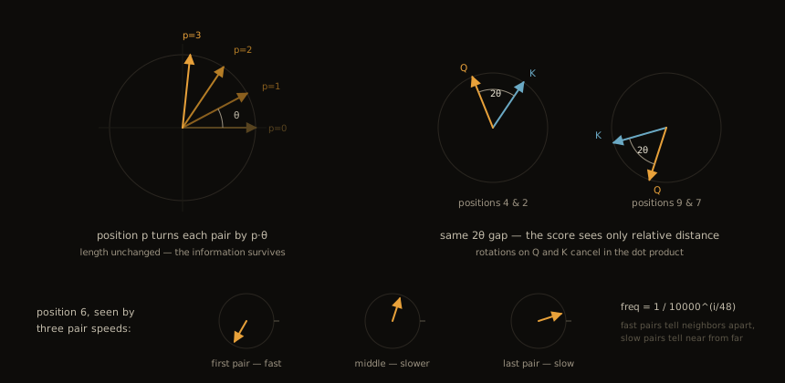
A head’s score is one big dot product over 48 numbers — which is simply a sum of 48 little products. A sum does not care how you group it. So group it two at a time, along the same pairs RoPE used: each bracket is then the first-float product plus the second-float product of one pair — which is exactly the dot product of that pair’s two arrows, query’s against key’s. The whole score is 24 arrow-to-arrow dot products, added up. Whatever we show about one pair of arrows is true for the score.

Look at one pair — say floats 0 and 1. The query has an arrow there, and the cached key has its own arrow there; their dot product is one bracket of the score. Both arrows were turned by RoPE: the query sits at position p, so its arrow was turned p steps of the pair’s angle theta; the key came from position q, so its arrow was turned q steps. A dot product only cares about lengths and the angle between the arrows — and rotation kept the lengths. The angle between them is now exactly their distance apart: (p - q) * theta. A key right behind the query was turned almost as far — small gap between the arrows. A key from long ago lags far behind — big gap. The absolute positions cancel: “three tokens ago” means the same gap at position 10 and at position 210.

One speed would not be enough: turn far enough and an arrow comes back to the start, and position 0 would look like position 6. So each of a head’s 24 pairs turns at its own speed, from one full turn every ~6 tokens down to a barely visible drift — the second, minute, and hour hands of a clock. That spread is the 1.0 / pow(10000.0, ...) line in rope; the base 10000 is a convention from the earliest transformers, and any wide spread of speeds works. V is never rotated. Rotation has one purpose — make the Q–K score feel distance. V never enters a score: it is what gets blended after the weights are already decided. Rotating it would add position where position is not wanted, and only scramble the value it returns.

def rope(var x : array<float>; position, head_size, size : int) {
    for (pair in range(size / 2)) {
        let i = pair * 2
        let frequency = 1.0 / pow(10000.0, float(i % head_size) / float(head_size))
        let angle = float(position) * frequency
        let a = x[i]
        let b = x[i + 1]
        let sin_angle = sin(angle)
        let cos_angle = cos(angle)
        x[i] = a * cos_angle - b * sin_angle
        x[i + 1] = a * sin_angle + b * cos_angle
    }
}

The rotated K and the untouched V are then appended to the layer’s KV cache: the model’s stored keys and values for every position it has processed, the current one included. This is the stored record from the prefill story — prefill filled it, and every generated token keeps adding to it. The cache is plain memoization — without it, every new token would recompute K and V for the entire past.

One more dial lives here. Some models cache fewer K/V heads than they have query heads (kv_heads in the code), and several query heads then share one cached head — a memory saver called grouped-query attention. kv_multiple = c.heads / c.kv_heads is that sharing factor; for stories15M it is 1 — every query head has its own cached head — and the code carries the general form.

Now the look-back itself. For one head and one cached position p, the code computes:

score[p] = dot(query, key_cache[p]) / sqrt(head_size)

A high score means “this cached position holds what I am looking for” — the query’s arrow agrees with that key’s arrow. The sqrt(head_size) division keeps scores in a fixed range at any width: 48 mostly-unrelated products partly cancel each other, and such a sum grows like sqrt(48), not like 48. The range matters for the next step.

softmax turns the head’s scores into attention weights: positive numbers that sum to one. It raises e to each score and divides by the total — exp(s[i] - max(s)) / sum(exp(s[j] - max(s))) — subtracting the largest score first, which changes no ratio but keeps exp from overflowing. The exponent is why the range mattered: scores a few units apart already produce a near-total winner, and unscaled scores would freeze every head into a hard single-position lookup instead of a soft blend. (Not the same “weights” as the model’s parameters — older texts use one word for both. Here, parameters live in the checkpoint; weights come out of softmax.)

def softmax(var x : array<float>; size : int) {
    var largest = x[0]
    for (i in range(1, size)) {
        largest = max(largest, x[i])
    }
    var sum = 0.0
    for (i in range(size)) {
        x[i] = exp(x[i] - largest)
        sum += x[i]
    }
    for (i in range(size)) {
        x[i] /= sum
    }
}

The weighted sum

attention_head = sum(weight[p] * value_cache[p])

is the retrieved information: mostly the values of high-scoring positions, faint traces of the rest.

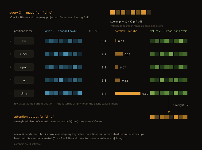
The score loop stops at the current position. Later positions are not in the cache — they do not exist yet — so the model cannot look ahead. This property has a name, the causal mask: causal as in cause and effect — the future must not influence the present. Here it costs nothing; it is simply the loop’s end.

The six 48-float head outputs are glued side by side — 288 again — and one more matrix, attention_output, mixes the six separate answers into a single 288-wide correction, which is added to x. This addition is the residual connection: the layer adds its finding and keeps everything it received:

x = x + attention(x)

8.7.1.6.3. Feed-forward: rework the token’s features

Attention moved information between positions. The second block works on the current token alone. Values flow one way through it — input, a wider middle, output, no loops, no looking sideways — and that is its name: the feed-forward block.

Its shape is: expand, gate, contract. After another RMSNorm, two matrices expand the 288-float stream to 768 values each. Think of a workbench: x is a tight 288-float summary, and the two matrices unpack it by asking 768 more learned questions of it — more questions than the stream itself can carry. Each of the 768 answers is one feature: how strongly x contains one learned pattern.

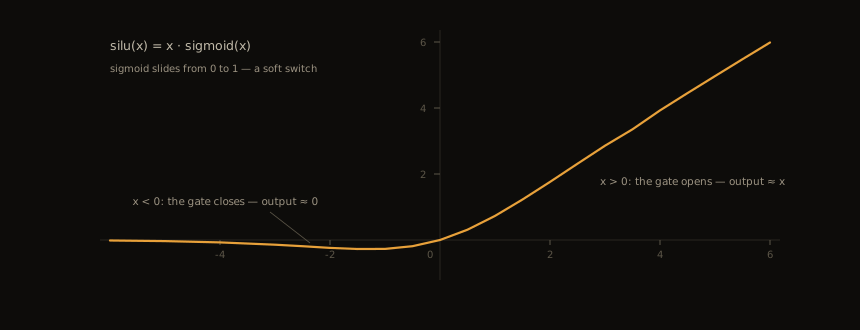
One of the two expanded copies goes through silu and becomes the gate for the other. SiLU — sigmoid linear unit — is x * sigmoid(x), where sigmoid(x) = 1 / (1 + exp(-x)) slides smoothly from 0 to 1: a soft switch. The code writes the product as one division:

def silu(var x : array<float>; size : int) {
    for (i in range(size)) {
        x[i] /= 1.0 + exp(-x[i])
    }
}

Why not simply x >= 0 ? x : 0? That function exists — ReLU — and it ruled for years. The problem is training. Training moves every number in tiny steps along slopes, and ReLU is exactly flat below zero: a feature pushed negative goes dead, no slope left to pull it back. SiLU never goes fully flat — slightly negative inputs keep a little signal and a little slope, so training can change its mind about them. It costs an exp and wins on quality; the SwiGLU paper famously admits it has no theory for why — it just measured better.

Most “why” questions on this page end the same way. Why 288 and not 300? Why six heads? Why base 10000? The shamans of the past tried different incantations, kept what worked, and we get to rationalize later why abra is so much better than cadabra. When this page gives a reason, the reason is real — but the numbers came first, and the explanations came after.

The two copies multiply element by element: where the gate is near zero, that feature is switched off; where it is large, the feature passes. A third matrix packs the 768 surviving answers back into 288 floats — the residual stream has one fixed width, and the correction has to be addable to x. The whole recipe:

hidden = W_down (SiLU(W_gate x) * (W_up x))
x      = x + hidden

This gated shape is commonly called SwiGLU (SiLU + gated linear unit). Why 768 and not some other number: it is a capacity dial, not a law — roughly 8/3 of dim, the ratio the Llama family settled on. Bigger would be more capacity and more compute.

The bend in the SiLU curve is what makes depth work at all. Two matrix multiplications in a row are exactly one — purely linear chains collapse. Put a bend between them and they stop collapsing: each layer can reshape what earlier layers made instead of restating it. The feed-forward block also holds about two thirds of every layer’s parameters, in these three matrices. The second residual addition closes the layer. Attention plus feed-forward, six times — the whole stack.

8.7.1.6.4. Logits: the vector becomes a choice

After the final layer, one last RMSNorm steadies x, and the classifier projects it from 288 values to 32,000 logits — one dot product of x against each row of the embedding table, one row per vocabulary token. The table has now been used both ways a grid of numbers can be used: at the start an ID indexed into it and picked one row; here x multiplies it, and every row answers at once. For stories15M these are literally the same numbers (shared_classifier in the code; larger models often train a separate matrix), so the question is literal: which token’s row does x now point along?

Stop on that question, because it is the heart of the whole page. x started as the current token’s own row — so why does the comparison name the token that comes after? Nothing in the arithmetic makes it so. It is what training selected every parameter to achieve: layer by layer, x is pushed away from “the token I am” and toward “the token that follows here”, because that final comparison is exactly what training scored, billions of times. The code on this page is the pipeline; the checkpoint’s numbers are why it points the right way.

most_likely picks the largest logit — this is called greedy decoding, and it is deterministic: one prompt, one story:

def most_likely(logits : array<float>) : int {
    var best = 0
    for (i in range(1, length(logits))) {
        if (logits[i] > logits[best]) {
            best = i
        }
    }
    return best
}

But we do not have to pick the top one every time. Turn the logits into probabilities with softmax, roll the dice, and every run can tell a different story. Choosing this way is called sampling, and the chat-UI knobs live here: temperature scales the logits before the softmax — higher means a wilder roll; top-p keeps only the most likely few in the roll.

8.7.1.7. Prompting is repeated forward

tokenizer.bin stores, for every token, its text piece and a precomputed merge score. encode begins with token 1 — BOS, beginning of sequence, written <s> in the figures: a marker the model saw at the start of every training text. Before the first word it also inserts the tokenizer’s leading-space token, because pieces mark word starts with a space. It then splits the prompt into UTF-8 characters, falling back to raw bytes for anything the vocabulary lacks (IDs 0–2 are reserved markers, so byte b lives at token b + 3), and then repeatedly joins the highest-scoring adjacent pair found in the vocabulary — the merge scores decide which pairs deserve to be one token. This is BPE — byte-pair encoding — in its SentencePiece flavor (SentencePiece is Google’s tokenizer scheme; llama2.c reuses its file format). token_text is the decoder half of the same scheme: pieces carry a leading space that marks a word start, which the first word after BOS drops, and <0xNN> pieces decode back to raw bytes.

Prefill is a plain loop:

for (position, token in range(length(tokens)), tokens) {
    forward(c, w, model, s, token, position)
}

After the last prompt token, state.logits already predicts the first completion token. Generation chooses it, prints its vocabulary piece, calls forward with that token at the next position, and repeats. The KV cache written during prefill keeps the whole prompt available to every generated token.

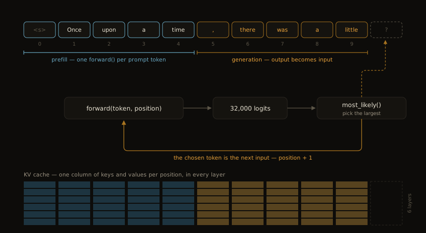
We prefill one token at a time so you can see it plainly; production dasLLAMA does batches, same result. Generation stops when the model predicts token 1 again: the training data was many stories laid end to end with the BOS marker between them, so predicting it is the model saying “this story is complete — a new one would start here.” The checkpoint’s sequence length is the other stop: the hard bound on how many positions the model can hold.

8.7.1.8. From seed to library

This program deliberately fixes everything to one tiny model: the dimensions, the file format, the precision, the execution strategy, the sampling policy. dasLLAMA is what happens when each of those constraints becomes an interface:

• the fixed layout becomes GGUF — the standard file format LLMs ship in — plus an architecture registry;

• fp32 matrices become quantized formats — parameters stored in fewer bits, so bigger models fit in the same memory — with tuned kernels;

• serial row loops become job-queue work;

• serial prompt prefill becomes a batched implementation;

• greedy choice becomes a sampling pipeline;

• one tokenizer becomes model-specific tokenization; and

• scratch arrays become reusable sessions with managed KV caches.

This happened fast. The first dasLLAMA commit was authored on 2026-06-27, and it began with the same naive fp32 matmul used on this page. About a day later, PR #3297 contained Llama-2 and Llama-3, GGUF loading, quantization, threading, batched prefill, tests, and chat. The path from this readable file to native machine code never had to leave one programming environment.

The important part is visible before any of that machinery: a fully functional transformer is small enough to read, run, interpret, JIT, and improve in one source file. That is the problem dasLLAMA solves at production scale.

8.7.1.9. Credits and further reading

This tutorial reimplements, in daslang, the design of Andrej Karpathy’s llama2.c: the checkpoint format, the tokenizer format, and the shape of the forward pass all follow his run.c. The checkpoint is his tinyllamas training run on the TinyStories dataset (Eldan & Li) — which is why a 15-million-parameter model can tell a coherent story at all.

If this page leaves you wanting the training half of the story, Karpathy teaches it better than anyone:

• Neural Networks: Zero to Hero — the full video course, from backpropagation to a working GPT;

• Let’s build GPT: from scratch, in code, spelled out — the transformer built live, the natural companion to this page;

• Let’s build the GPT Tokenizer — everything encode glosses over.

The architecture itself comes from the papers: Attention Is All You Need (the transformer), RoFormer (rotary position embedding), GLU Variants Improve Transformer (SwiGLU), and Llama 2 (this exact assembly of them).

See also

Full source: tutorials/dasLLAMA/00_problem_statement.das

Next tutorial: dasLLAMA-01 — Hello, Generation